Reproduce

You can reproduce our classification control experiments from our preprint by following these instructions.

The big overview (as described in our paper) is:

1. Train an SAE on the ImageNet-1K patch activations from a CLIP ViT-B/16, from the 11th (second-to-last) layer.
2. Show that you get meaningful features, through visualizations.
3. Train a linear probe on the [CLS] token activations from a CLIP ViT-B/16, from the 12th layer, on the Caltech-101 dataset. We use an arbitrary random train/test split.
4. Show that we get good accuracy.
5. Manipulate the activations using the proposed SAE features.
6. Be amazed. :)

To do these steps:

Record ImageNet-1K activations

Train an SAE on Activations

uv run python -m saev train \
  --sweep configs/preprint/classification.toml \
  --data.shard-root /local/scratch/$USER/cache/saev/ac89246f1934b45e2f0487298aebe36ad998b6bd252d880c0c9ec5de78d793c8/ \
  --data.layer -2 \
  --sae.d-vit 768

Visualize the SAE Features

`` was the best checkpoint from my sweep.

uv run python -m saev visuals \
  --ckpt checkpoints/bd97z80b/sae.pt \
  --dump-to /research/nfs_su_809/workspace/stevens.994/saev/features/bd97z80b \
  --sort-by patch \
  --data.shard-root /local/scratch/stevens.994/cache/saev/ac89246f1934b45e2f0487298aebe36ad998b6bd252d880c0c9ec5de78d793c8/ \
  --data.layer -2 \
  --log-freq-range -2.5 -1.5 \
  --log-value-range 0.0 1.0 \
  images:imagenet-dataset

You can see some neat features in here by using saev.interactive.features with marimo.

Record CUB-200-2011 Activations

For each $SPLIT in "train" and "test":

uv run python -m saev activations \
  --model-family clip \
  --model-ckpt ViT-B-16/openai \
  --d-vit 768 \
  --n-patches-per-img 196 \
  --layers -2 -1 \
  --dump-to /local/scratch/$USER/cache/saev \
  --n-patches-per-shard 2_4000_000 \
  data:image-folder-dataset \
  --data.root /nfs/datasets/caltech-101/$SPLIT

Train a Linear Probe

uv run python -m contrib.classification \
  --n-workers 32 \
  --train-imgs.root /research/nfs_su_809/workspace/stevens.994/datasets/cub2011/train \
  --val-imgs.root /research/nfs_su_809/workspace/stevens.994/datasets/cub2011/test/ \
  --sweep contrib/classification/sweep.toml
  ```

Then look at `logs/contrib/classification/hparam-sweeps.png`. 
It probably works for any of the learning rates above 1e-5 or so.

## Manipulate

Now we will manipulate the inputs to the probe by using the directions proposed by the SAE trained on ImageNet-1K and observe the changes in the linear model's predictions.
There are two ways to do this:

1. The marimo dashboard, which requires that you run your own inference.
2. The online dashboard, which is more polished but offers less control.

Since you have gone through the effort of training all this stuff, you probably want more control and have the hardware for inference.

Run the marimo dashboard with:

```sh
uv run marimo edit contrib/classification/interactive.py

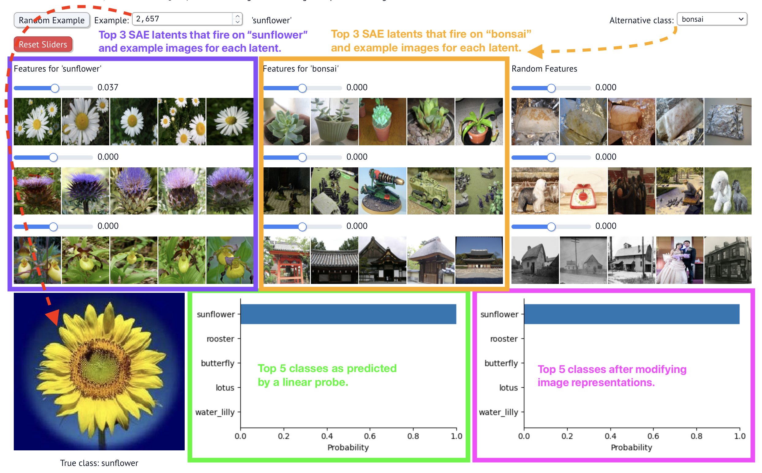
These screenshots show the kinds of findings you can uncover with this dashboard.

First, when you open the dashboard and configure the options, you will eventually see something like this:

The main parts of the dashboard:

1. Example selector: choose which test image to classify. The image is shown on the bottom left.
2. The top SAE latents for the test image's class (in purple below). The latent values of $h$ are also shown. Many will be 0 because SAE latents fire very rarely (sparse autoencoder).
3. The top SAE latents for another, user-selected class (in orange below). Choose the class on the top right dropdown.
4. The top classes as predicted by the pre-trained classification model (a linear probe; shown in green below).
5. The top classes as predicted by the same pre-trained classification model, after modifying the dense vector representation with the SAE's vectors. These predictions are updated as you change the sliders on the screen.

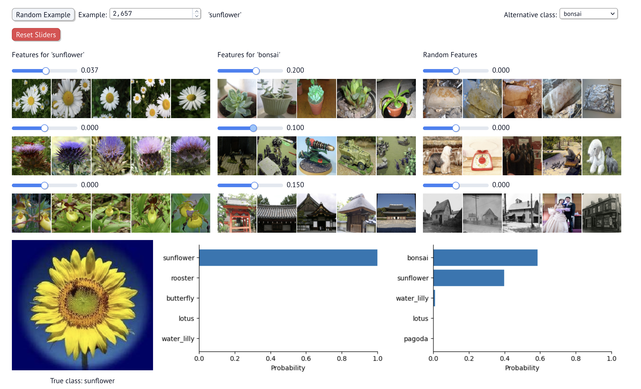
As an example, you can scale up the top bonsai features. As you do, the most likely class will be a bonsai. See below.

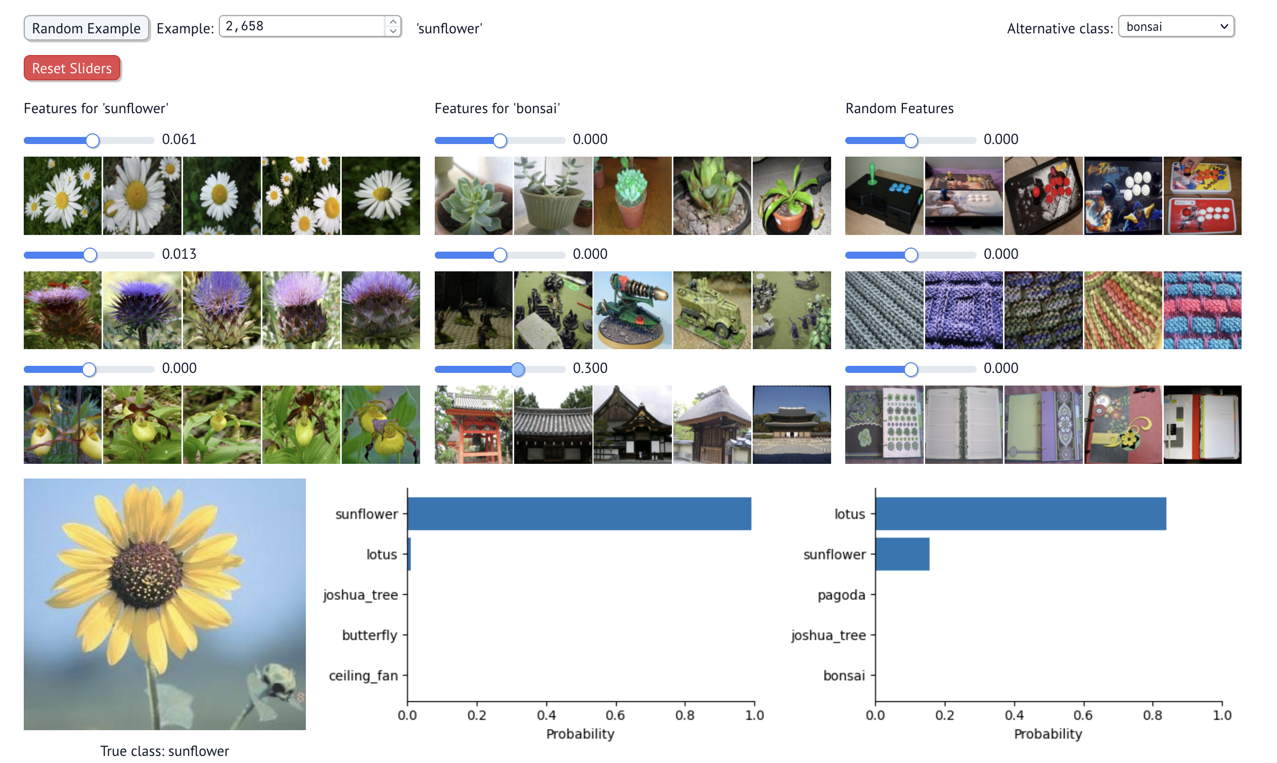
Here's another example. With another sunflower, you can manipulate turn up the SAE feature that fires strongly on pagodas and other traditionally Asian architectural structures. If you do, the most likley classification is a lotus, which is popular in Japanese and other Asian cultures.

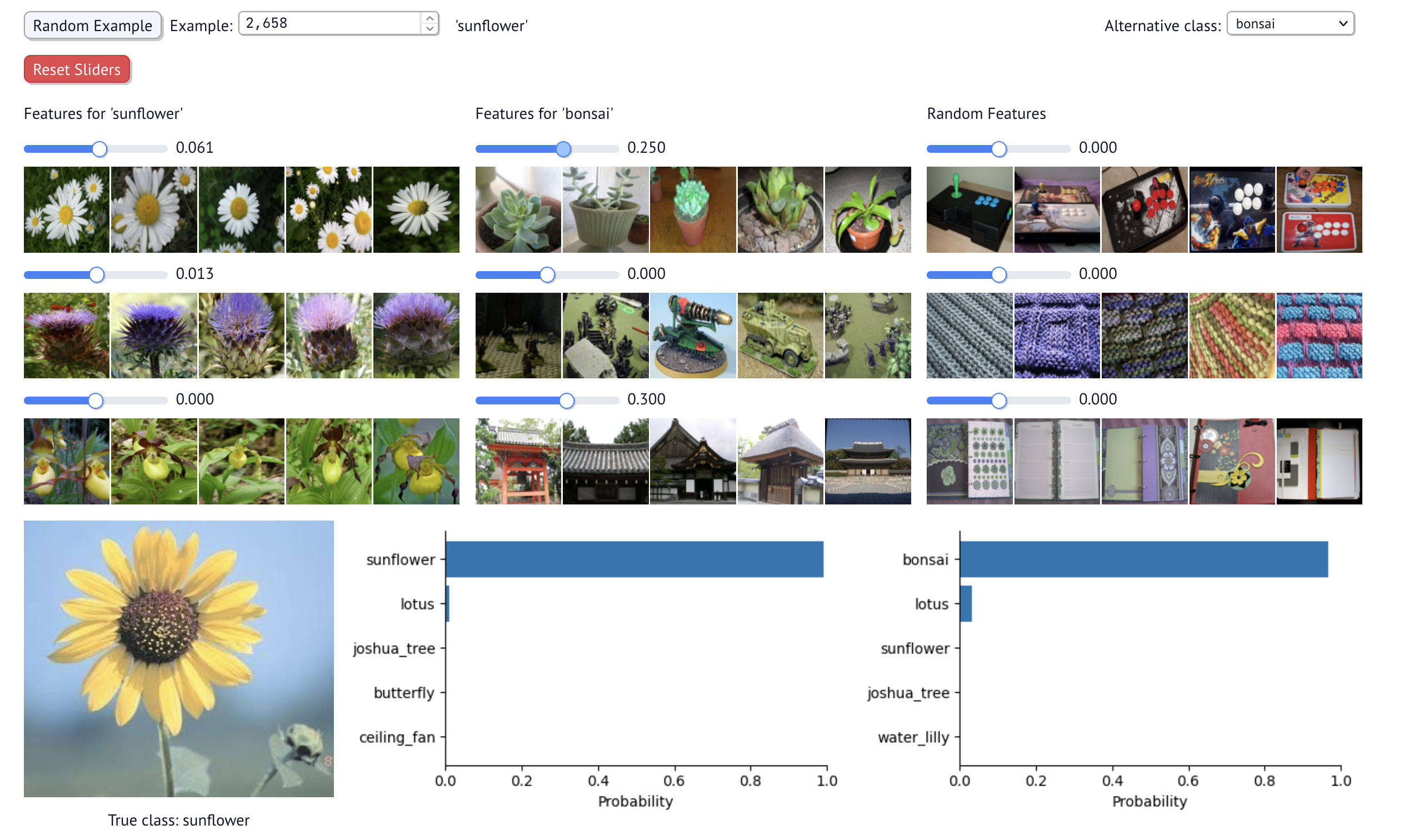
Only once you turn up the SAE feature that fires strongly on potted plants does the classification change to bonsai (which are typically potted).

I encourage you to look at other test images and manipulate the predictions!

Make Figures

uv run scripts/preprint/make_figures.py classification \
  --probs-before "Blue Jay" 0.49 "Clark\nNutcracker" 0.15 "White-Breasted\nNuthatch" 0.11 "Florida\nJay" 0.07 \
  --probs-after "Clark\nNutcracker" 0.31 "White-Breasted\nNuthatch" 0.19 "Great Grey\nShrike" 0.11 "Blue Jay" 0.10

Sub-modules

contrib.classification.config

contrib.classification.download_caltech101

A script to download the Caltech101 dataset for use as an saev.activations.ImageFolderDataset …

contrib.classification.download_cub

contrib.classification.download_flowers

A script to download the Flowers102 dataset …

contrib.classification.interactive

contrib.classification.plot_logits

Generates plots demonstrating SAE feature specificity in image classification …

contrib.classification.training

Train a linear probe on [CLS] activations from a ViT.